Gallery

A tour of what pyplotrs can draw. Every entry below is a complete, runnable script — copy it, run it, and you get the figure shown. (Scripts live in examples/ and save a PNG into the current directory.)

• Line
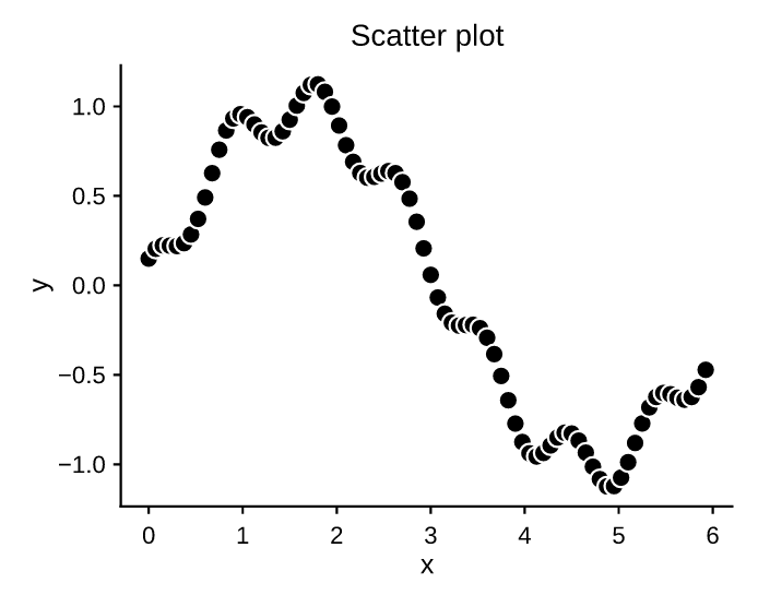• Scatter
• Bar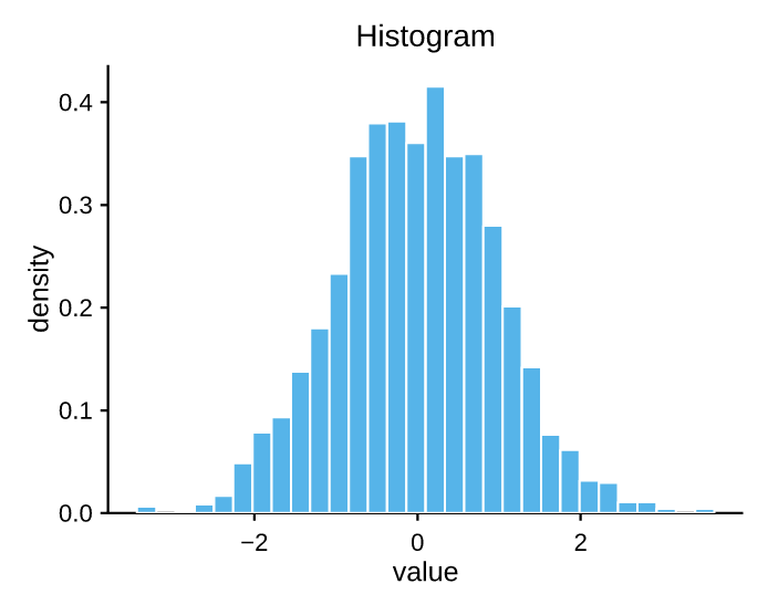
• Histogram
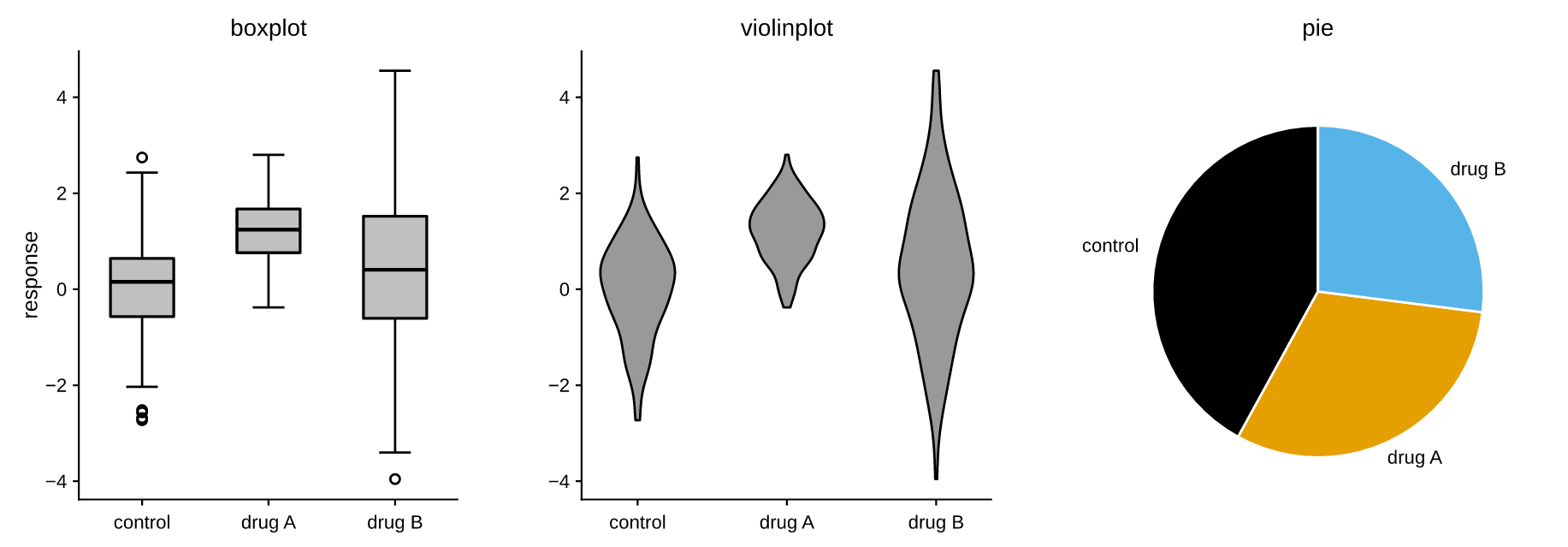• Box / violin / pie
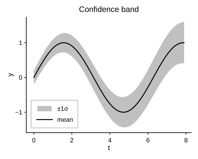• Fill between
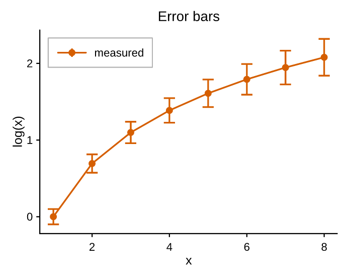• Error bars
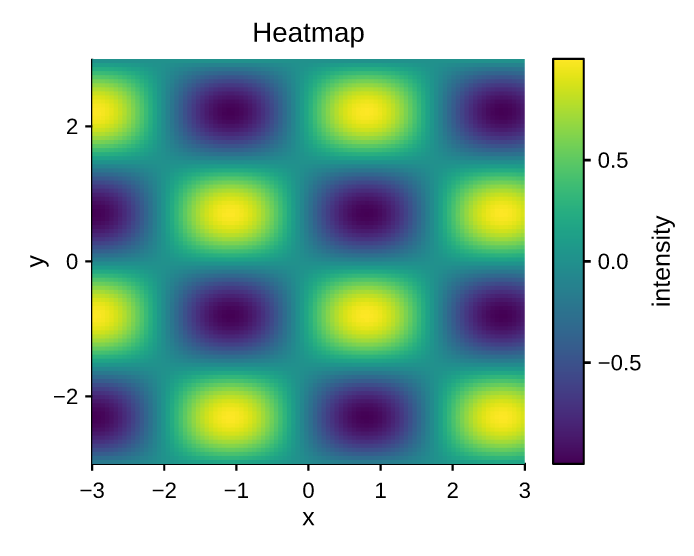• Heatmap
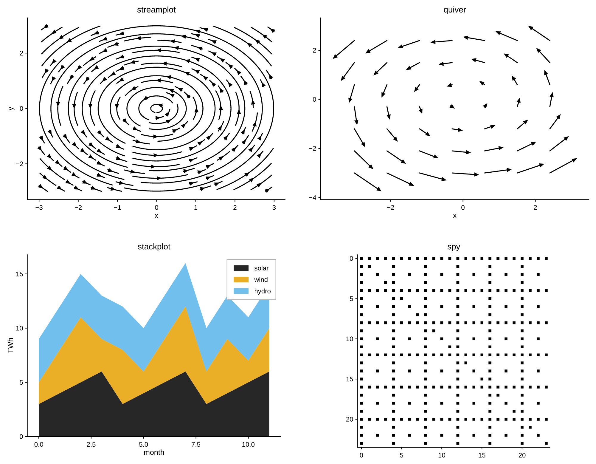• Fields
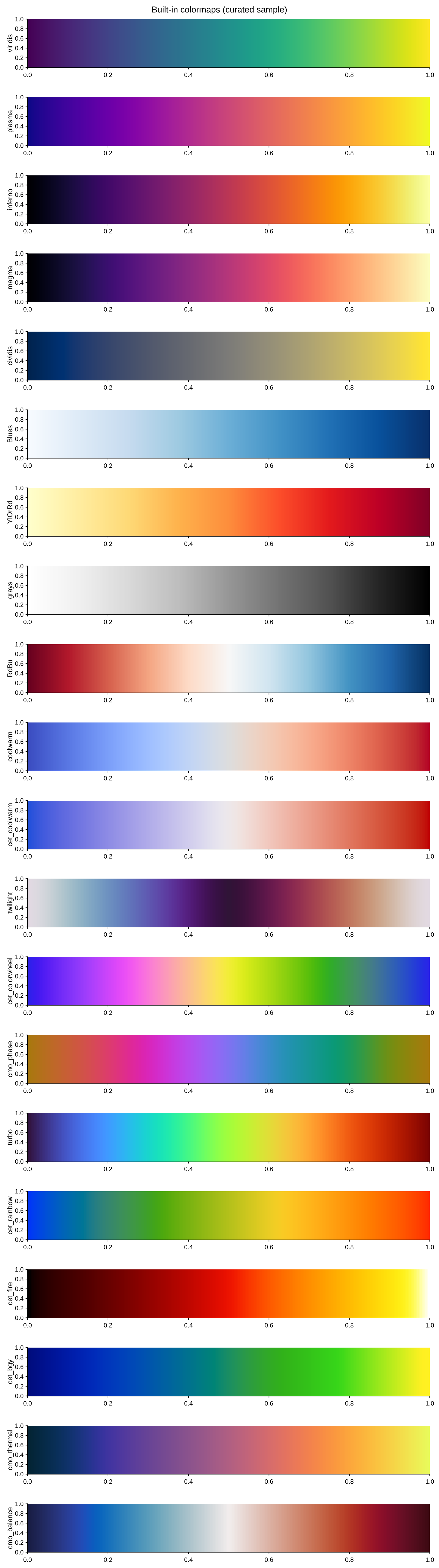• Colormaps
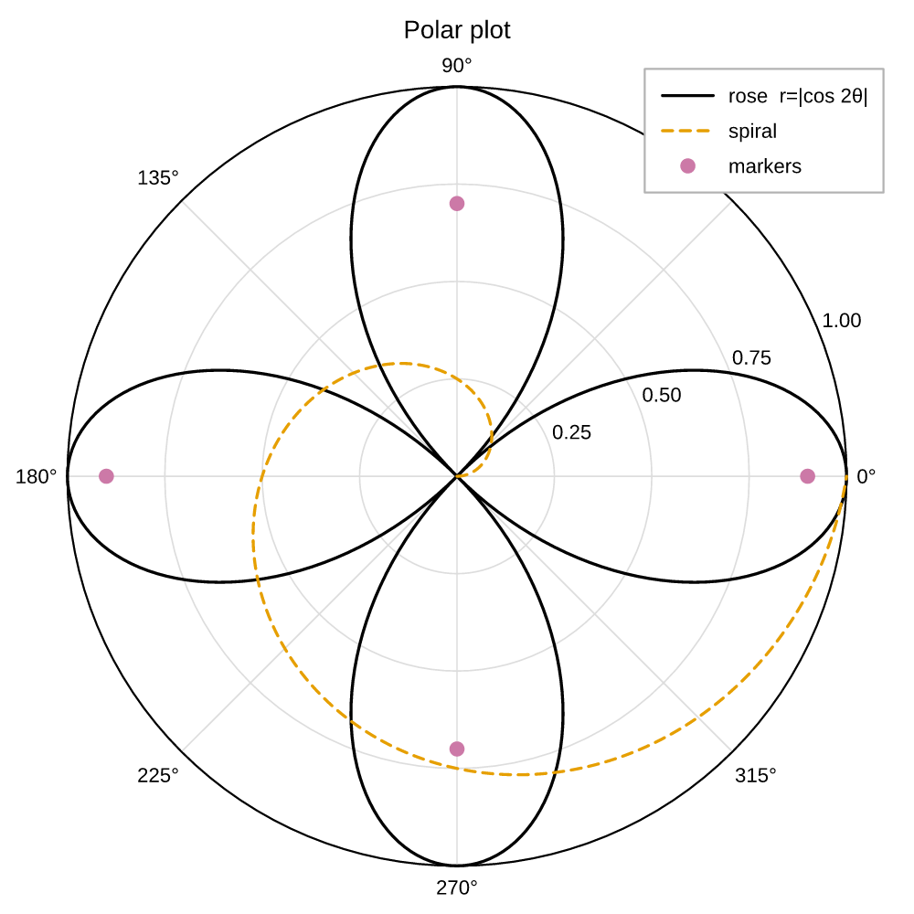• Polar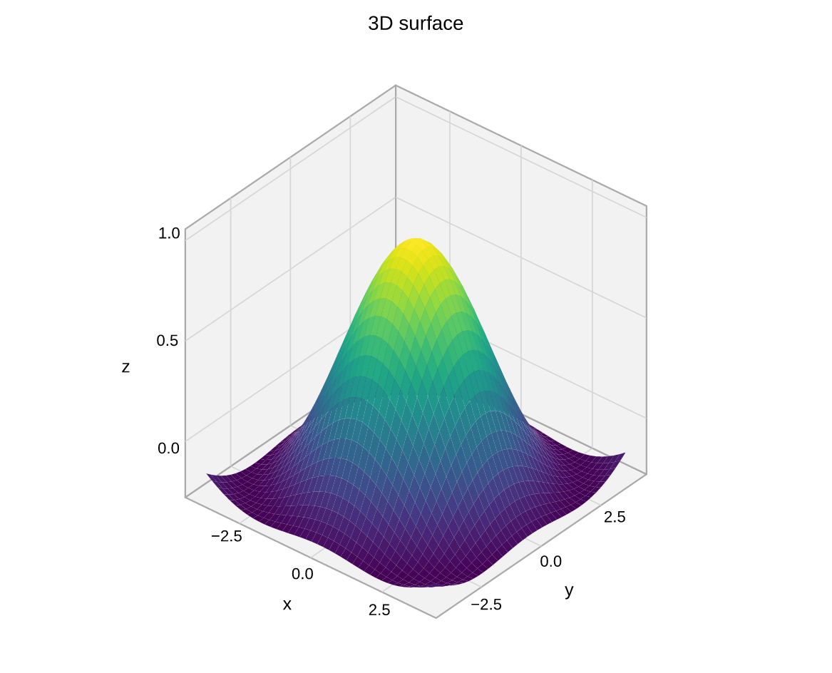
• 3D surface
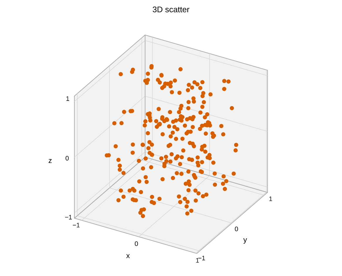• 3D scatter
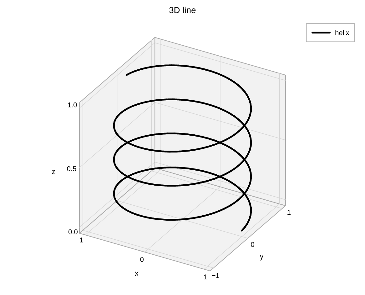• 3D line
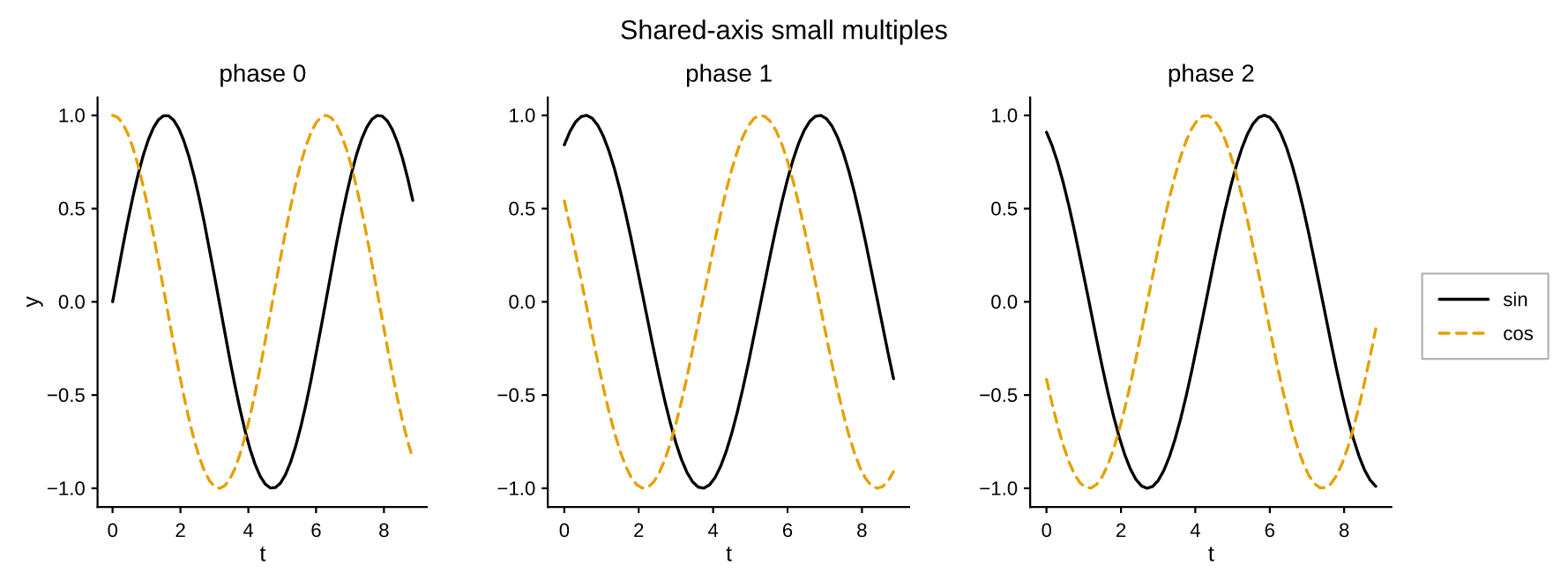• Subplots
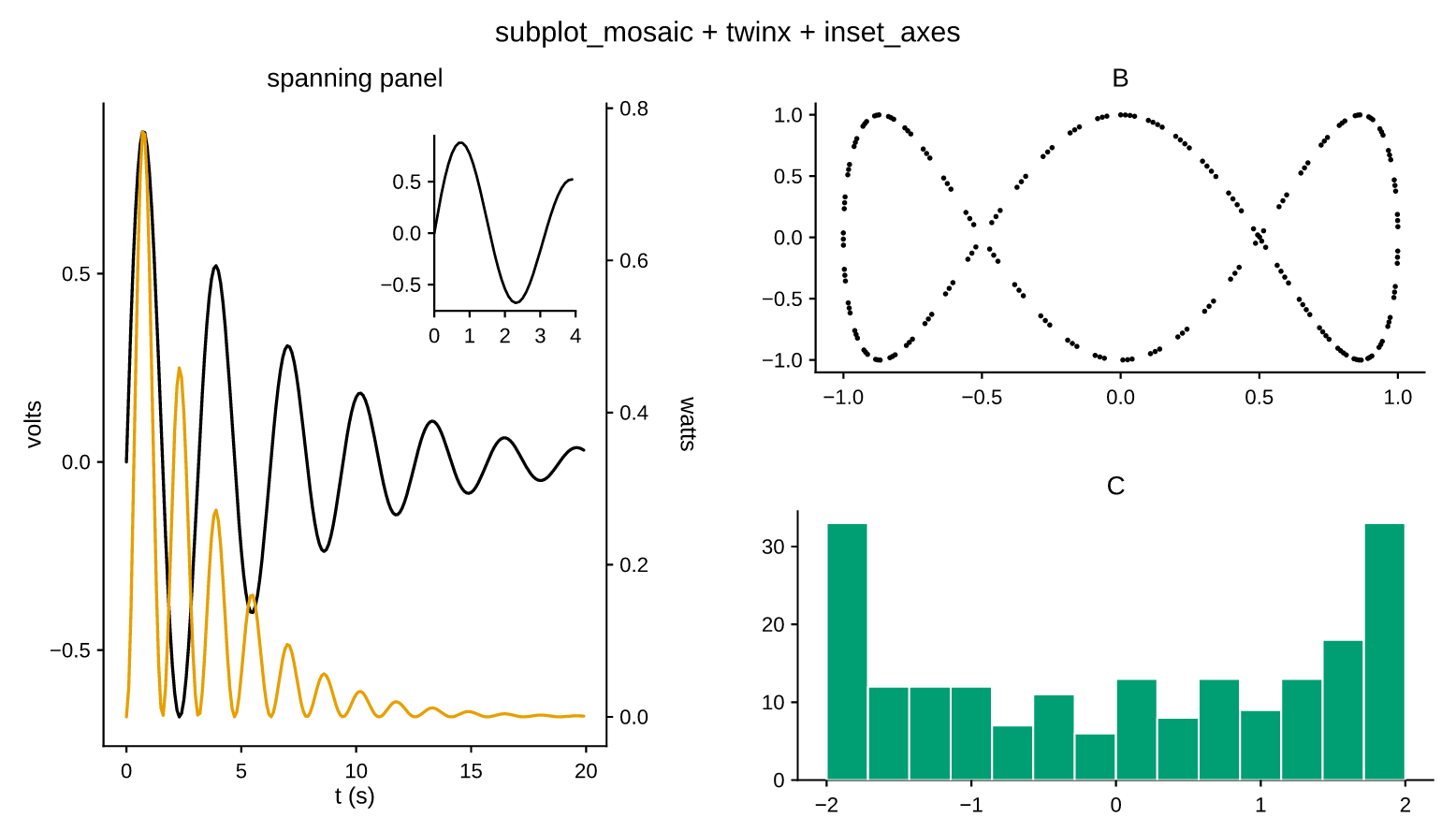• Mosaic & insets
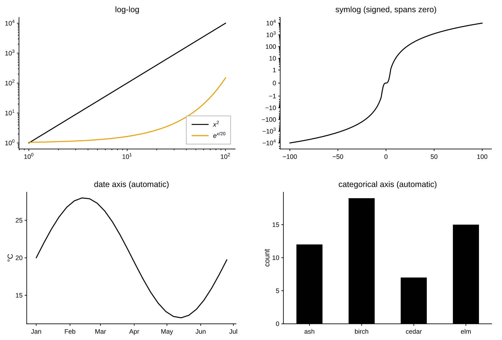• Axis scales
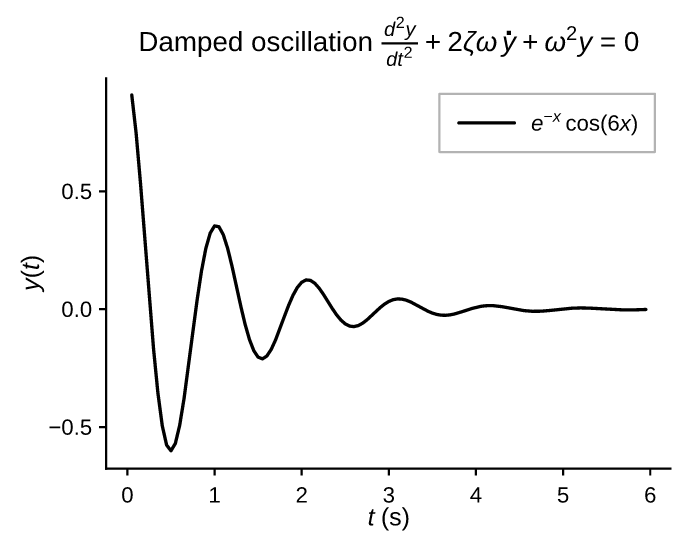• LaTeX math
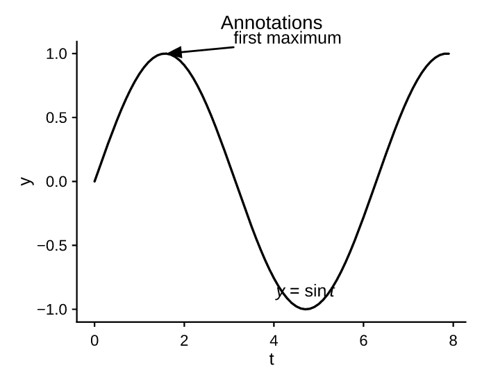• Annotations
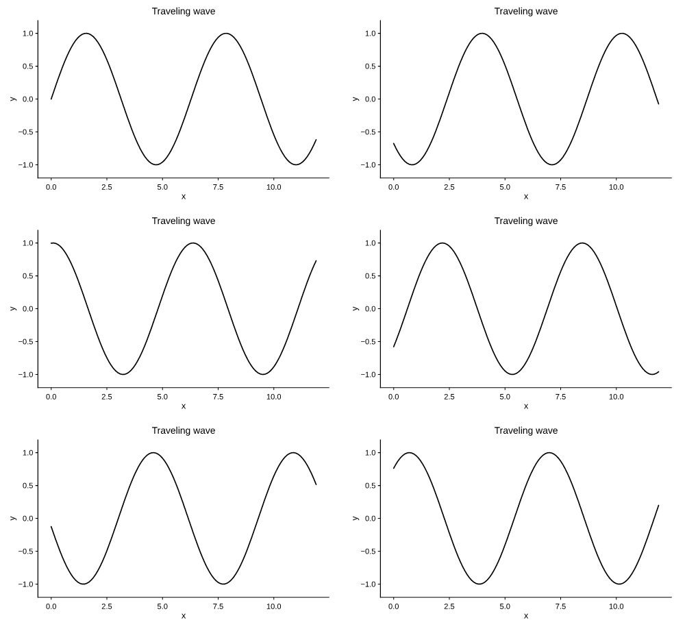• Animation

---

Basic plots

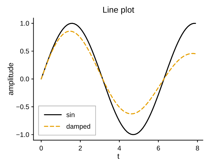
Line plot

"""Line plot: multiple series with a legend."""
import math

import pyplotrs as pp

xs = [i * 0.1 for i in range(80)]
fig, ax = pp.subplots()
ax.line(xs, [math.sin(x) for x in xs], label="sin")
ax.line(xs, [math.sin(x) * math.exp(-0.1 * x) for x in xs],
        label="damped", linestyle="dashed")
ax.set(title="Line plot", xlabel="t", ylabel="amplitude")
ax.legend()
fig.save("line.png")

Scatter

"""Scatter plot with marker styling."""
import math

import pyplotrs as pp

n = 80
xs = [i / n * 6 for i in range(n)]
ys = [math.sin(x) + 0.15 * math.cos(7 * x) for x in xs]
fig, ax = pp.subplots()
ax.scatter(xs, ys, markersize=6.3, marker="o", color="C0",
           edgecolor=(255, 255, 255, 255), edgewidth=0.8)
ax.set(title="Scatter plot", xlabel="x", ylabel="y")
fig.save("scatter.png")

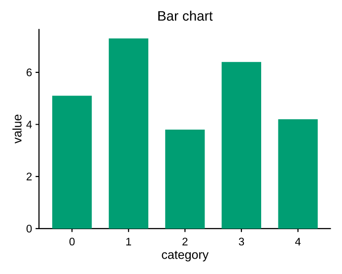
Bar chart

"""Vertical bar chart."""
import pyplotrs as pp

x = [0, 1, 2, 3, 4]
heights = [5.1, 7.3, 3.8, 6.4, 4.2]
fig, ax = pp.subplots()
ax.bar(x, heights, width=0.7, color="C3")
ax.set(title="Bar chart", xlabel="category", ylabel="value")
fig.save("bar.png")

---

Distributions

Histogram

"""Histogram of a synthetic distribution."""
import math

import pyplotrs as pp


# Box-Muller normal samples (no numpy dependency).
def normals(n, seed=1):
    s = seed
    out = []
    for _ in range(n):
        s = (1103515245 * s + 12345) & 0x7FFFFFFF
        u1 = (s + 1) / 0x80000000
        s = (1103515245 * s + 12345) & 0x7FFFFFFF
        u2 = (s + 1) / 0x80000000
        out.append(math.sqrt(-2 * math.log(u1)) * math.cos(2 * math.pi * u2))
    return out

fig, ax = pp.subplots()
ax.hist(normals(2000), bins=30, color="C2", density=True)
ax.set(title="Histogram", xlabel="value", ylabel="density")
fig.save("histogram.png")

Box, violin and pie

"""Distribution marks: boxplot, violinplot, and a labeled pie."""
import math
import random

import pyplotrs as pp

random.seed(7)
groups = [[random.gauss(mu, sd) for _ in range(200)]
          for mu, sd in [(0.0, 1.0), (1.2, 0.6), (0.4, 1.6)]]
labels = ["control", "drug A", "drug B"]

fig, (ax_box, ax_violin, ax_pie) = pp.subplots(1, 3, figsize=(660, 230))

ax_box.boxplot(groups)
ax_box.set(title="boxplot", ylabel="response", xticks=[1, 2, 3], xticklabels=labels)

ax_violin.violinplot(groups)
ax_violin.set(title="violinplot", xticks=[1, 2, 3], xticklabels=labels)

ax_pie.pie([42, 31, 27], labels=labels)
ax_pie.set(title="pie")

fig.save("statistical.png")

Fill between

"""Fill between curves: a line with a confidence band."""
import math

import pyplotrs as pp

xs = [i * 0.1 for i in range(80)]
mid = [math.sin(x) for x in xs]
lo = [m - 0.2 - 0.05 * x for m, x in zip(mid, xs)]
hi = [m + 0.2 + 0.05 * x for m, x in zip(mid, xs)]
fig, ax = pp.subplots()
ax.fill_between(xs, lo, hi, color="C0", alpha=0.25, label="±1σ")
ax.line(xs, mid, color="C0", label="mean")
ax.set(title="Confidence band", xlabel="t", ylabel="y")
ax.legend()
fig.save("fill_between.png")

Error bars

"""Error bars with caps."""
import math

import pyplotrs as pp

xs = list(range(1, 9))
ys = [math.log(x) for x in xs]
yerr = [0.08 + 0.02 * x for x in xs]
fig, ax = pp.subplots()
ax.errorbar(xs, ys, yerr=yerr, marker="o", capsize=4, color="C6", label="measured")
ax.set(title="Error bars", xlabel="x", ylabel="log(x)")
ax.legend()
fig.save("errorbar.png")

---

Images & colormaps

Heatmap

"""Image / heatmap with a colorbar."""
import math

import pyplotrs as pp

n = 100
data = [[math.sin(i / 8) * math.cos(j / 10) for j in range(n)] for i in range(n)]
fig, ax = pp.subplots()
m = ax.imshow(data, cmap="viridis", extent=(-3, 3, -3, 3))
fig.colorbar(m, label="intensity")
ax.set(title="Heatmap", xlabel="x", ylabel="y")
fig.save("heatmap.png")

Vector and matrix fields

"""Vector-field and matrix plot types: quiver, streamplot, stackplot, spy."""

import pyplotrs as pp

N = 21
xc = [-3 + 6 * j / (N - 1) for j in range(N)]
yc = [-3 + 6 * i / (N - 1) for i in range(N)]
# Solid-body rotation: u = -y, v = x.
U = [[-yc[i] for _ in range(N)] for i in range(N)]
V = [[xc[j] for j in range(N)] for _ in range(N)]

fig, axes = pp.subplots(nrows=2, ncols=2, figsize=(720, 560))
(ax_stream, ax_quiver), (ax_stack, ax_spy) = axes

ax_stream.streamplot(xc, yc, U, V, density=1.1)
ax_stream.set(title="streamplot", xlabel="x", ylabel="y")

step = 3
ax_quiver.quiver(
    [xc[::step] for _ in yc[::step]],
    [[y] * len(xc[::step]) for y in yc[::step]],
    [[-yc[i] for j in range(0, N, step)] for i in range(0, N, step)],
    [[xc[j] for j in range(0, N, step)] for i in range(0, N, step)],
    scale=0.25,
)
ax_quiver.set(title="quiver", xlabel="x")

months = list(range(12))
ax_stack.stackplot(
    months,
    [3 + i % 4 for i in months],
    [2 + (i * 2) % 5 for i in months],
    [4 + (i * 3) % 3 for i in months],
    labels=["solar", "wind", "hydro"],
    alpha=0.85,
)
ax_stack.set(title="stackplot", xlabel="month", ylabel="TWh")
ax_stack.legend()

sparse = [[1 if (i * j) % 4 == 0 or i == j else 0 for j in range(24)] for i in range(24)]
ax_spy.spy(sparse, markersize=3.5)
ax_spy.set(title="spy")

fig.save("fields.png")

Colormaps

"""A reference strip across the built-in colormap families (a curated sample
- see ``colormaps.available()`` for the full set of ~125)."""
import pyplotrs as pp

# perceptually uniform, sequential, diverging, cyclic, miscellaneous, then one
# representative pull from each third-party source (colorcet `cet_`, cmocean `cmo_`).
names = [
    "viridis", "plasma", "inferno", "magma", "cividis",
    "Blues", "YlOrRd", "grays",
    "RdBu", "coolwarm", "cet_coolwarm",
    "twilight", "cet_colorwheel", "cmo_phase",
    "turbo", "cet_rainbow",
    "cet_fire", "cet_bgy",
    "cmo_thermal", "cmo_balance",
]
strip = [[j / 255 for j in range(256)] for _ in range(8)]
fig, axs = pp.subplots(len(names), 1, figsize=(560, 100 * len(names)))
for ax, name in zip(axs, names):
    ax.imshow(strip, cmap=name, extent=(0, 1, 0, 1))
    ax.set(ylabel=name)
fig.set(suptitle="Built-in colormaps (curated sample)")
fig.save("colormaps.png")

---

Polar

Polar

"""Polar plot: line + scatter on a polar projection, with a legend."""
import math

import pyplotrs as pp

theta = [i * math.pi / 180 for i in range(0, 361)]
fig, ax = pp.subplots(projection="polar", figsize=(360, 360))
ax.plot(theta, [abs(math.cos(2 * t)) for t in theta], label="rose  r=|cos 2θ|")
ax.plot(theta, [t / (2 * math.pi) for t in theta], label="spiral", linestyle="dashed")
ax.scatter([0, math.pi / 2, math.pi, 3 * math.pi / 2], [0.9, 0.7, 0.9, 0.7],
           color="C7", label="markers")
ax.set(title="Polar plot")
ax.legend(loc="upper right")
fig.save("polar.png")

---

3D

3D surface

"""3D surface (the classic 'sombrero')."""
import math

import pyplotrs as pp

n = 40
xs = [-4 + 8 * i / (n - 1) for i in range(n)]
ys = [-4 + 8 * j / (n - 1) for j in range(n)]
X = [[x for x in xs] for _ in ys]
Y = [[y for _ in xs] for y in ys]
def f(x, y):
    r = math.sqrt(x * x + y * y) + 1e-6
    return math.sin(r) / r
Z = [[f(x, y) for x in xs] for y in ys]
fig, ax = pp.subplots(projection="3d", figsize=(420, 340))
ax.surface(X, Y, Z, cmap="viridis")
ax.set(title="3D surface", xlabel="x", ylabel="y", zlabel="z", elev=35, azim=-50)
fig.save("surface3d.png")

3D scatter

"""3D scatter cloud."""
import math

import pyplotrs as pp


def rnd(seed):
    s = seed
    while True:
        s = (1103515245 * s + 12345) & 0x7FFFFFFF
        yield (s / 0x7FFFFFFF) * 2 - 1
g = rnd(7)
xs, ys, zs = [], [], []
for _ in range(220):
    t = next(g) * math.pi
    r = 0.6 + 0.4 * next(g)
    xs.append(r * math.cos(3 * t) + 0.1 * next(g))
    ys.append(r * math.sin(3 * t) + 0.1 * next(g))
    zs.append(t / math.pi)
fig, ax = pp.subplots(projection="3d", figsize=(420, 340))
ax.scatter(xs, ys, zs, color="C6", markersize=5.1)
ax.set(title="3D scatter", xlabel="x", ylabel="y", zlabel="z")
fig.save("scatter3d.png")

3D line

"""A 3D parametric curve (helix)."""
import math

import pyplotrs as pp

t = [i * 0.1 for i in range(220)]
xs = [math.cos(v) for v in t]
ys = [math.sin(v) for v in t]
zs = [v / (22.0) for v in t]
fig, ax = pp.subplots(projection="3d", figsize=(420, 340))
ax.plot(xs, ys, zs, color="C0", linewidth=2.0, label="helix")
ax.set(title="3D line", xlabel="x", ylabel="y", zlabel="z")
ax.legend()
fig.save("line3d.png")

---

Layout & styling

Subplots

"""A multi-panel figure with a shared y-axis and a figure-level legend."""
import math

import pyplotrs as pp

xs = [i * 0.15 for i in range(60)]
fig, axs = pp.subplots(1, 3, figsize=(640, 240), sharey=True)
for k, ax in enumerate(axs):
    ax.line(xs, [math.sin(x + k) for x in xs], label="sin")
    ax.line(xs, [math.cos(x + k) for x in xs], label="cos", linestyle="dashed")
    ax.set(title=f"phase {k}", xlabel="t")
axs[0].set(ylabel="y")
fig.legend()
fig.set(suptitle="Shared-axis small multiples")
fig.save("subplots.png")

Mosaic, twin axis and inset

"""Layout tools: a mosaic of spanning panels, a twin y-axis, and an inset."""
import math

import pyplotrs as pp

fig, axd = pp.subplot_mosaic(
    """
    AB
    AC
    """,
    figsize=(560, 320),
)

xs = [i * 0.1 for i in range(200)]

# A spans both rows: a decaying signal with a second series in other units.
signal = [math.exp(-x / 6) * math.sin(2 * x) for x in xs]
axd["A"].line(xs, signal, label="signal (V)")
axd["A"].set(title="spanning panel", xlabel="t (s)", ylabel="volts")

power = axd["A"].twinx()
power.line(xs, [s * s for s in signal], color="C1", label="power (W)")
power.set(ylabel="watts")

# An inset zooms the first oscillation of the same trace.
zoom = axd["A"].inset_axes((0.55, 0.62, 0.4, 0.33))
zoom.line(xs[:40], signal[:40], linewidth=1.0)
zoom.set(xlim=(0, 4))

axd["B"].scatter([math.sin(x) for x in xs], [math.cos(3 * x) for x in xs], markersize=2)
axd["B"].set(title="B")

axd["C"].hist([math.sin(x) * 2 for x in xs], bins=14, color="C3")
axd["C"].set(title="C")

fig.set(suptitle="subplot_mosaic + twinx + inset_axes")
fig.save("layout.png")

Axis scales

"""Axis scales: log, symlog, an automatic date axis, and categories."""
import datetime as dt
import math

import pyplotrs as pp

fig, ((ax_log, ax_symlog), (ax_date, ax_cat)) = pp.subplots(2, 2, figsize=(620, 420))

xs = [1 + i * 0.5 for i in range(200)]
ax_log.line(xs, [x ** 2 for x in xs], label="$x^2$")
ax_log.line(xs, [math.exp(x / 20) for x in xs], label="$e^{x/20}$")
ax_log.set(title="log-log", xscale="log", yscale="log")
ax_log.legend(loc="lower right")

ts = [-100 + i for i in range(201)]
ax_symlog.line(ts, [t ** 3 / 100 for t in ts])
ax_symlog.set(title="symlog (signed, spans zero)", yscale="symlog")

# Datetime values switch that axis to a date scale automatically; the
# formatter here just shortens the auto labels from "Jan 2026" to "Jan".
day0 = dt.date(2026, 1, 1)
days = [day0 + dt.timedelta(days=7 * i) for i in range(26)]
ax_date.line(days, [20 + 8 * math.sin(i / 4) for i in range(26)])
ax_date.set(title="date axis (automatic)", ylabel="°C",
            xformatter=pp.ticker.DateFormatter("%b"))

# String coordinates switch that axis to a categorical scale.
ax_cat.bar(["ash", "birch", "cedar", "elm"], [12, 19, 7, 15])
ax_cat.set(title="categorical axis (automatic)", ylabel="count")

fig.save("scales.png")

Themes

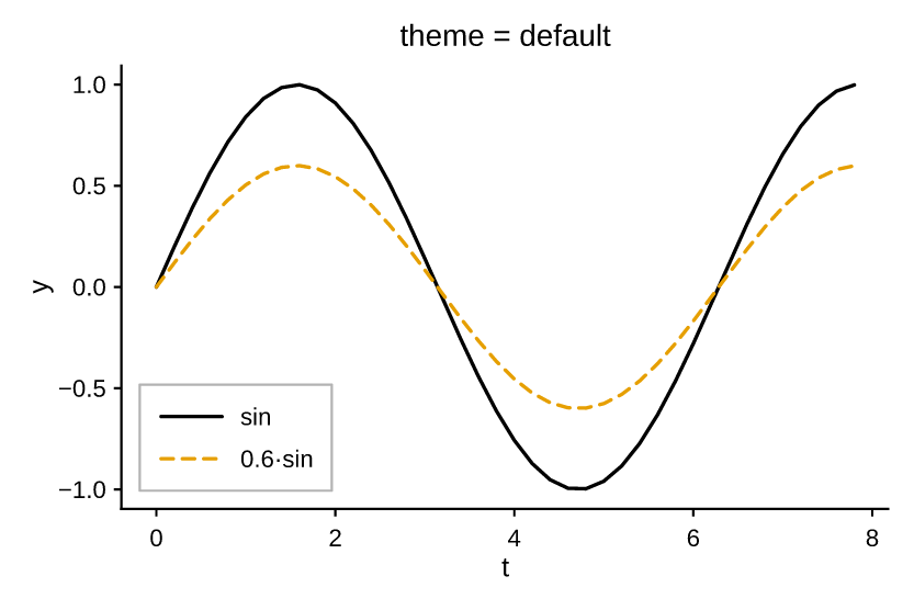
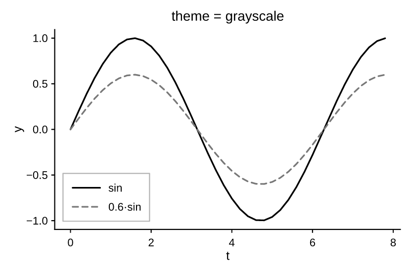
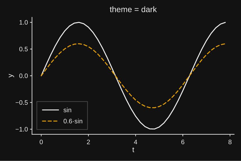
"""Built-in themes: one figure per preset, shown together.

A theme is passed to ``subplots`` and flows to its axes (there is no global
'current theme'). Here we render the same line in each preset.
"""
import math

import pyplotrs as pp

xs = [i * 0.2 for i in range(40)]
ys = [math.sin(x) for x in xs]
for name in ["default", "grayscale", "dark"]:
    fig, ax = pp.subplots(figsize=(300, 200), theme=name)
    ax.line(xs, ys, label="sin")
    ax.line(xs, [y * 0.6 for y in ys], label="0.6·sin", linestyle="dashed")
    ax.set(title=f"theme = {name}", xlabel="t", ylabel="y")
    ax.legend()
    fig.save(f"theme_{name}.png")

---

Math & annotations

LaTeX math

"""LaTeX math in titles, axis labels and the legend."""
import math

import pyplotrs as pp

xs = [i * 0.05 for i in range(1, 120)]
fig, ax = pp.subplots()
ax.line(xs, [math.exp(-x) * math.cos(6 * x) for x in xs],
        label=r"$e^{-x}\cos(6x)$")
ax.set(title=r"Damped oscillation $\frac{d^2y}{dt^2}+2\zeta\omega\,\dot y+\omega^2 y=0$",
       xlabel=r"$t\ \mathrm{(s)}$", ylabel=r"$y(t)$")
ax.legend()
fig.save("math_labels.png")

Annotations

"""Text and callout-arrow annotations in data coordinates."""
import math

import pyplotrs as pp

xs = [i * 0.1 for i in range(80)]
ys = [math.sin(x) for x in xs]
peak = max(range(len(xs)), key=lambda i: ys[i])
fig, ax = pp.subplots()
ax.line(xs, ys, color="C0")
ax.annotate("first maximum", (xs[peak], ys[peak]),
            xytext=(xs[peak] + 1.5, ys[peak] + 0.05))
ax.text(4.7, -0.9, r"$y=\sin t$", ha="center", color="C0")
ax.set(title="Annotations", xlabel="t", ylabel="y")
fig.save("annotations.png")

---

Animation

Animation

"""An animated GIF: a traveling wave."""
import math

import pyplotrs as pp

xs = [i * 0.1 for i in range(120)]

def frame(i):
    fig, ax = pp.subplots(figsize=(360, 220))
    ax.line(xs, [math.sin(x - i * 0.3) for x in xs], color="C0")
    ax.set(title="Traveling wave", xlabel="x", ylabel="y", ylim=(-1.2, 1.2))
    return fig

pp.animate(frame, frames=40, fps=20).save("animation_wave.gif")