Math & annotations

LaTeX math

Any text — titles, axis labels, tick labels, legend entries, annotations — may contain $...$ math. It is typeset by a faithful, MathJax-grade engine driven by the math font's OpenType MATH table, and stays real, selectable text in the PDF/SVG output (copy-paste yields the Unicode math).

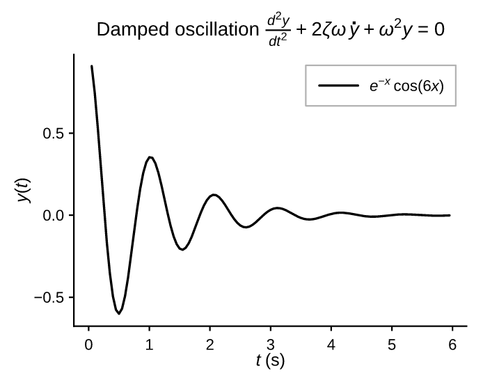
"""LaTeX math in titles, axis labels and the legend."""
import math

import pyplotrs as pp

xs = [i * 0.05 for i in range(1, 120)]
fig, ax = pp.subplots()
ax.line(xs, [math.exp(-x) * math.cos(6 * x) for x in xs],
        label=r"$e^{-x}\cos(6x)$")
ax.set(title=r"Damped oscillation $\frac{d^2y}{dt^2}+2\zeta\omega\,\dot y+\omega^2 y=0$",
       xlabel=r"$t\ \mathrm{(s)}$", ylabel=r"$y(t)$")
ax.legend()
fig.save("math_labels.png")

Supported syntax includes:

• super/subscripts ^ _ (and both on one nucleus, x_0^2);
• {...} grouping;
• \frac{a}{b}, \binom{n}{k};
• \sqrt{...} and \sqrt[n]{...} (a stretchy radical);
• auto-sized \left...\right fences;
• a broad Greek / operator / relation / arrow table (\alpha, \sum, \int, \leq, \to, \infty, \partial, …);
• accents \hat, \bar, \vec, \tilde, \dot, \ddot, …;
• math alphabets \mathbf, \mathit, \mathbb, \mathcal, \mathfrak, \mathsf, \mathtt, …;
• \text{...} and \operatorname{...} for upright runs.

Raw strings

Write math labels as raw strings (r"$\alpha$") so Python doesn't interpret the backslashes.

When you save to HTML and a label contains $...$, the math is re-rendered by an inlined copy of MathJax (SVG output), so it stays selectable and you can right-click → Show Math As to copy the LaTeX/MathML — fully offline.

Math in a tick label works too, which is how a log axis writes its decades as $10^{k}$ — see LogFormatter.

Which face draws what

Math is set in your own body family, wherever that family has the glyphs. Variables and Greek come from its italic, digits and upright roman from the face the label itself is in, and the common operators (+ − × · ÷ / = < > ≤ ≥ ≠ ≈ ( ) [ ] ∂ ∞ → …) from the same place. So $\sin\omega t$ is Arial throughout, and a bold title's math is bold throughout — variables included.

What your family cannot supply are the parts that have to grow: a radical sized to its content, a \left(...\right) fence sized to what it wraps, a \sum enlarged in display style. Growing a glyph needs the variant and assembly chains of an OpenType MATH table, and no text font has one. Those come from Fira Math, a bundled sans math font (175 KB) — so √, ∑ and ∫ are monoline marks that match Arial, not the high-contrast Times shapes a serif math font draws.

Between the two sit two more fallbacks, each reached only when the one before it has no glyph:

• a DejaVu Sans subset (95 KB) for symbols neither your family nor Fira Math carries. Text families cover the symbol blocks raggedly — Arial has → ← ↔ but not ⇒ ⇐ ↦, ∩ but not ∪, ≤ ≥ ≠ ≈ but not ≪ ≫ ∝ ∼ — so without it a single expression could set $A \cap B$ sans and $A \cup B$ serif;
• STIX Two Math last, for the Script and Fraktur alphabets (\mathcal, \mathfrak) and double-struck digits, which no sans math font here has. Those are calligraphic letterforms by definition, so a serif source is the right one.

Positioning constants always come from the primary math font, whichever face ends up drawing a given mark, so a span is laid out to one font's metrics.

This is the same line matplotlib's default dejavusans set draws, for the same reason: a label is read against its neighbors. Drawing math wholly from a serif math font made a log axis label 10³ Times while the y ticks beside it read 50 and 100 in Arial — and, less obviously, made $E = mc^2$ mix a serif E m c with a sans = and 2.

Two consequences worth knowing:

• Most figures embed no math font at all — the math fonts are reached only for something that grows or for a symbol your family lacks.
• Math follows set_font_family. Set Helvetica and your variables are Helvetica Italic.

Uniformly serif math

To set every atom in STIX Two Math instead — the traditional look, and what you want when the body text is a serif too:

pyplotrs.set_mathtext_fontset("stix")
pyplotrs.set_font_family("STIX Two Text", "Times New Roman")

set_mathtext_fontset("sans") (the default) restores the behavior above. It is pyplotrs' analog of matplotlib's rcParams["mathtext.fontset"].

HTML export

Saving to .html re-renders math with MathJax, which carries its own (serif) TeX fonts, so an HTML figure's math will not match a sans PNG or PDF of the same figure. Everything else on the page still matches.

Styling part of a label

weight=/style= apply to a whole label. To style a substring — one bold number, one tinted word, one highlighted term — build the label with rich and its shorthands instead of passing a string:

import pyplotrs as pp

ax.set(title=pp.rich("Growth ", pp.bold("+42%", color="teal"),
                     " over ", pp.italic("6 months")))

These work anywhere a label does: title, xlabel/ylabel, suptitle, xticklabels, a mark's label=, text and annotate.

Helper	Effect
pp.rich(*parts, **style)	the general span; with no style, just a container
pp.bold(...), pp.italic(...)	a real face of the body family, not a synthetic slant
pp.underline(...), pp.strike(...)	a rule from the face's own metrics
pp.mark(...)	a highlight panel behind the run
pp.plain(label)	the styling stripped back off, as a plain string

Style keys are weight, style, color, bgcolor, underline, strike, and either scale (a multiple of the label's own size — usually what you want, since a title and a tick label are set at different sizes) or size (absolute points). Colors accept everything the rest of the library does, "C0" palette indices included.

Spans nest, and an inner style wins over an outer one, so a run can opt back out of what encloses it:

pp.bold("all of this ", pp.rich("except this", weight="normal", color="#888"))

Rich text and math

A span may contain $...$, and the span's weight and slant become the ambient face the math is set in — so the math comes out bold throughout, variables included, rather than half-bold:

ax.set(title=pp.rich("fitted ", pp.bold(r"$E = mc^2$")))

To color inside a single expression, use \textcolor and \colorbox, which take any color spelling the rest of the library takes:

ax.set(xlabel=r"$\textcolor{C1}{\sigma} / \sqrt{N}$")
ax.set(title=r"minimize $\colorbox{#ffe89a}{\frac{a}{b}} + c$")

Emphasis within math has a second spelling that means something different: $\mathbf{v}$ selects the math alphabet (an upright bold vector), while pp.bold("$v$") changes the face the whole span is set in. Reach for the alphabet when the boldness is part of the notation, and for the span when it is part of the typography.

Kerning at a style boundary

Each run is shaped separately, so a kern pair straddling a style change is lost — pp.rich("W", pp.bold("a")) sets a hair wider than "Wa". Adjacent runs that share a style are merged back into one, so this costs you nothing where the style does not actually change.

Text annotations

text draws a string at data coordinates:

ax.text(2.5, 0.8, r"region of interest", ha="center", color="C1")
ax.text(0.1, 0.9, "N = 42", weight="bold", style="italic", fontsize=8)
ax.text(0.5, 0.5, "sideways", rotation=90)

Argument	Meaning
ha	left (default) / center / right
va	baseline (default) / bottom / center / top
color	defaults to the theme's text color
fontsize	in points; defaults to the theme's label size
weight, style	normal/bold and normal/italic — a real face, not a synthetic slant
rotation	degrees counter-clockwise about the anchor

Rotation is applied as a group transform in the output rather than baked into paths, so rotated text stays selectable in PDF and SVG.

Callout arrows

annotate points text at a data location, optionally with an arrow from the text to the point:

"""Text and callout-arrow annotations in data coordinates."""
import math

import pyplotrs as pp

xs = [i * 0.1 for i in range(80)]
ys = [math.sin(x) for x in xs]
peak = max(range(len(xs)), key=lambda i: ys[i])
fig, ax = pp.subplots()
ax.line(xs, ys, color="C0")
ax.annotate("first maximum", (xs[peak], ys[peak]),
            xytext=(xs[peak] + 1.5, ys[peak] + 0.05))
ax.text(4.7, -0.9, r"$y=\sin t$", ha="center", color="C0")
ax.set(title="Annotations", xlabel="t", ylabel="y")
fig.save("annotations.png")

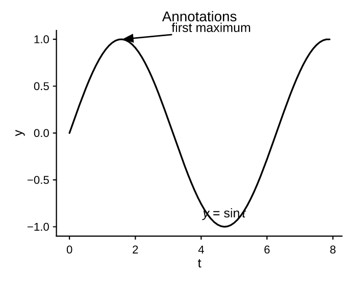
xy is the point being annotated and xytext is where the label sits (defaults to xy). Set arrow=False for a plain floating label. Both coordinates are in data space, the same ha/va/weight/style/rotation arguments apply, and the text may itself contain $...$ math.

Annotations do not move the view

Text and callouts are drawn over the data and take no part in autoscaling, so a label placed outside the data range will be clipped rather than stretching the axes to fit. Set xlim/ylim if you need room for it.