Layout

Figures & axes covered the regular subplots grid. This page covers everything past it: uneven grids, panels that span cells, axes placed inside other axes, and second axes stacked on the same cell.

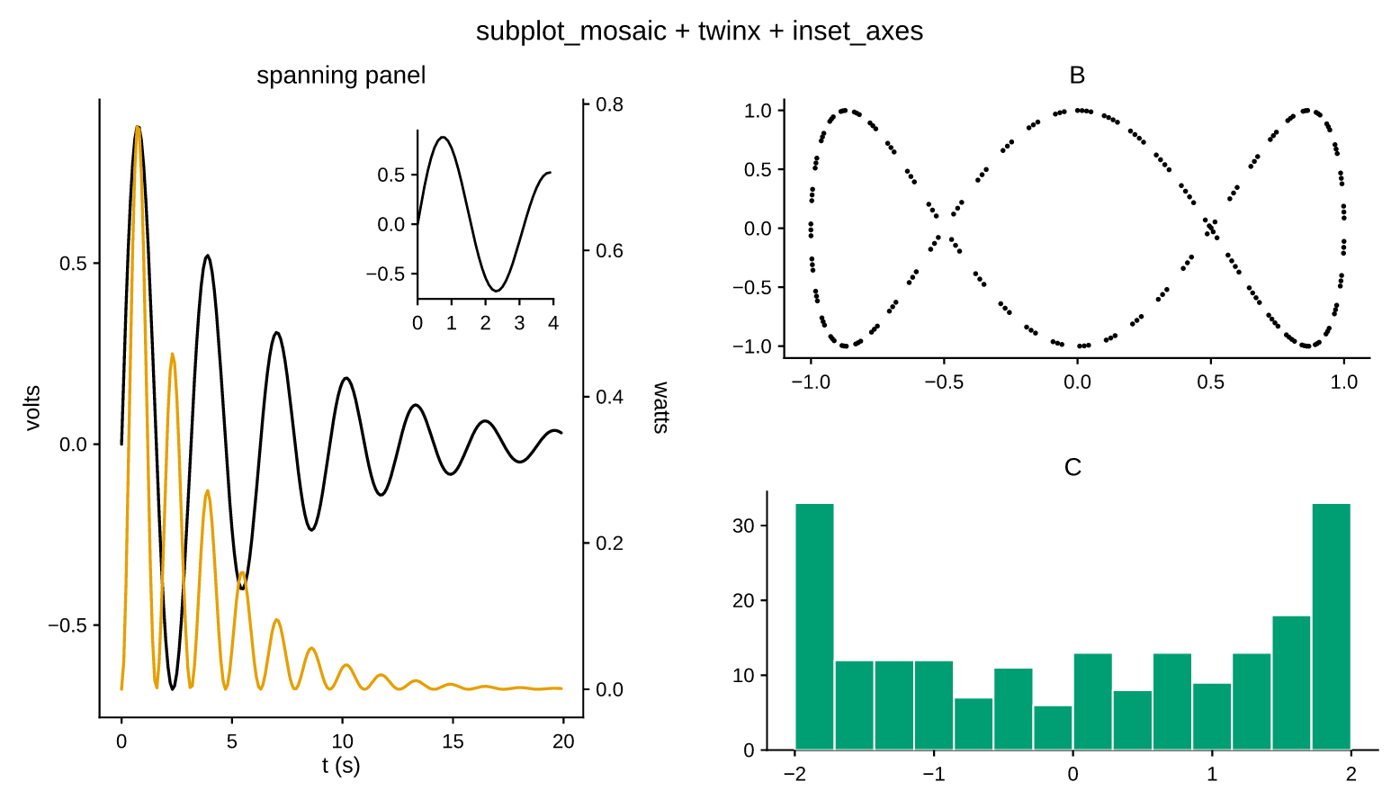
"""Layout tools: a mosaic of spanning panels, a twin y-axis, and an inset."""
import math

import pyplotrs as pp

fig, axd = pp.subplot_mosaic(
    """
    AB
    AC
    """,
    figsize=(560, 320),
)

xs = [i * 0.1 for i in range(200)]

# A spans both rows: a decaying signal with a second series in other units.
signal = [math.exp(-x / 6) * math.sin(2 * x) for x in xs]
axd["A"].line(xs, signal, label="signal (V)")
axd["A"].set(title="spanning panel", xlabel="t (s)", ylabel="volts")

power = axd["A"].twinx()
power.line(xs, [s * s for s in signal], color="C1", label="power (W)")
power.set(ylabel="watts")

# An inset zooms the first oscillation of the same trace.
zoom = axd["A"].inset_axes((0.55, 0.62, 0.4, 0.33))
zoom.line(xs[:40], signal[:40], linewidth=1.0)
zoom.set(xlim=(0, 4))

axd["B"].scatter([math.sin(x) for x in xs], [math.cos(3 * x) for x in xs], markersize=2)
axd["B"].set(title="B")

axd["C"].hist([math.sin(x) * 2 for x in xs], bins=14, color="C3")
axd["C"].set(title="C")

fig.set(suptitle="subplot_mosaic + twinx + inset_axes")
fig.save("layout.png")

Uneven grids

width_ratios and height_ratios weight the columns and rows:

fig, axs = pp.subplots(1, 2, width_ratios=[3, 1])   # wide panel, narrow panel
fig, axs = pp.subplots(2, 1, height_ratios=[3, 1])  # plot over a residual strip

Only the proportions matter — [3, 1] and [0.75, 0.25] are the same — and the gutters keep their size, so weighting changes the panels rather than the space between them. A malformed hint (wrong length, zero or negative) falls back to an even grid instead of raising.

Spanning panels: subplot_mosaic

An ASCII drawing of the layout is usually clearer than index arithmetic. subplot_mosaic takes one and hands back a dict keyed by the labels:

fig, axd = pp.subplot_mosaic(
    """
    AAB
    AAC
    .DC
    """
)
axd["A"].line(xs, ys)
axd["D"].hist(samples)

A spans the top-left 2×2 block, C spans two rows of the right column, and . (or a space) leaves a cell empty. Each label's cells must form a solid rectangle. The string is dedented before it is read, so the indented triple-quoted form above means what it looks like.

Spanning panels: GridSpec

The index-based route, for when the geometry is computed rather than drawn. Figure.add_gridspec returns a GridSpec you slice NumPy-style, and add_subplot places an axes on the slice:

fig = pp.figure(figsize=(500, 320))
gs = fig.add_gridspec(2, 3, height_ratios=[2, 1])

main  = fig.add_subplot(gs[0, :2])     # top-left, two columns wide
side  = fig.add_subplot(gs[:, 2])      # full-height right column
under = fig.add_subplot(gs[1, 0])
polar = fig.add_subplot(gs[1, 1], projection="polar")

pp.figure() creates a figure with no axes, which is what you want when every panel is placed by hand. add_subplot takes the same projection argument as subplots, so a single figure can mix 2D, polar and 3D panels.

Shared axes

sharex / sharey unify the data range across all panels, so they line up and are directly comparable:

fig, axs = pp.subplots(1, 3, sharey=True)
for k, ax in enumerate(axs):
    ax.line(xs, [f(x, k) for x in xs])

Sharing affects the range, not the chrome: each panel still draws its own ticks and tick labels. On stacked panels that duplication is usually unwanted, and blanking the inner labels is one argument:

top.set(xticklabels=[])    # keep the ticks, drop their labels

Every getter reports the shared result, so axs[0].get_ylim() on a sharey figure returns the range the whole row settled on.

Twin axes

twinx returns a second axes over the same cell, sharing the x-axis with an independent y-axis drawn on the right — the usual way to put two quantities in different units on one panel. twiny is the transpose.

fig, ax = pp.subplots()
ax.line(t, voltage, label="V")
ax.set(xlabel="t (s)", ylabel="volts")

power = ax.twinx()
power.line(t, watts, color="C1", label="W")
power.set(ylabel="watts")

The twin continues the palette rather than restarting it, so the second series does not silently come out the same color as the first. Plot on the object twinx() returned; the original ax still owns the left axis.

Insets

inset_axes places a child axes inside the parent's plot area, in fractions of that area ((0, 0) is the lower-left corner):

zoom = ax.inset_axes((0.55, 0.6, 0.4, 0.35))   # x0, y0, width, height
zoom.line(xs[:40], ys[:40])
zoom.set(xlim=(0, 4))

The inset is an ordinary Axes — its own scales, ticks, theme colors and marks.

Secondary axes

A secondary axis is a relabeling of the same data in another unit, not another set of data. secondary_xaxis / secondary_yaxis take a (forward, inverse) pair mapping primary values to secondary ones:

ax.set(xlabel="wavelength (nm)")
ax.secondary_xaxis("top",
                   functions=(lambda nm: 1239.8 / nm, lambda ev: 1239.8 / ev),
                   label="photon energy (eV)")

Omit functions for a plain duplicate axis on the far side. Unlike twinx, this returns the original axes, because there is nothing new to plot on.

Figure-level chrome

A Figure can carry a super-title, one shared legend, and colorbars:

fig.set(suptitle="An overview")
fig.legend(loc="right", ncol=2, title="condition")

Figure.legend collects the labeled marks of every panel — 2D, polar and 3D — de-duplicated by label, into a reserved column to the right of the grid. Because the column is part of the layout rather than an overlay, a figure legend can never cover data, and the panels shrink to make room for it. An Axes.legend sits inside its panel instead, and loc="best" scores each corner by how much data the box would cover.

Colorbars work the same way — see colormaps & images.

What the layout engine guarantees

Panels are solved in a single pass in Rust: every band a figure needs — titles, tick labels, axis labels, colorbar strips, the legend column — is reserved before anything is drawn, from the measured extent of the text that will go in it. There is no tight_layout to call and no iterative shrink-to-fit, which is also why the per-panel cost stays flat as the grid grows (see performance).