3D plots¶

pyplotrs' 3D support is a projection layer, not a separate renderer: an orthographic camera turns 3D primitives into ordinary 2D paths and text (with painter's-algorithm depth sorting), which then flow through the same PDF/SVG/PNG backends as everything else. The practical upshot is that 3D figures keep real editable text and stay fully vector — a surface exports as vector quads, not a rasterized image.

Make every axes of a figure 3D with projection="3d" (or a single panel with add_subplot(spec, projection="3d")):

import pyplotrs as pp

fig, ax = pp.subplots(projection="3d")

Surfaces¶

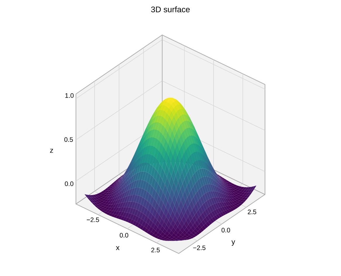
surface draws a colormapped surface over a grid (X, Y, Z). Z is a 2D nrows × ncols grid; X/Y may be matching 2D grids or 1D coordinate vectors that are broadcast.

"""3D surface (the classic 'sombrero')."""
import math

import pyplotrs as pp

n = 40
xs = [-4 + 8 * i / (n - 1) for i in range(n)]
ys = [-4 + 8 * j / (n - 1) for j in range(n)]
X = [[x for x in xs] for _ in ys]
Y = [[y for _ in xs] for y in ys]
def f(x, y):
    r = math.sqrt(x * x + y * y) + 1e-6
    return math.sin(r) / r
Z = [[f(x, y) for x in xs] for y in ys]
fig, ax = pp.subplots(projection="3d", figsize=(420, 340))
ax.surface(X, Y, Z, cmap="viridis")
ax.set(title="3D surface", xlabel="x", ylabel="y", zlabel="z", elev=35, azim=-50)
fig.save("surface3d.png")

3D surface

Lines¶

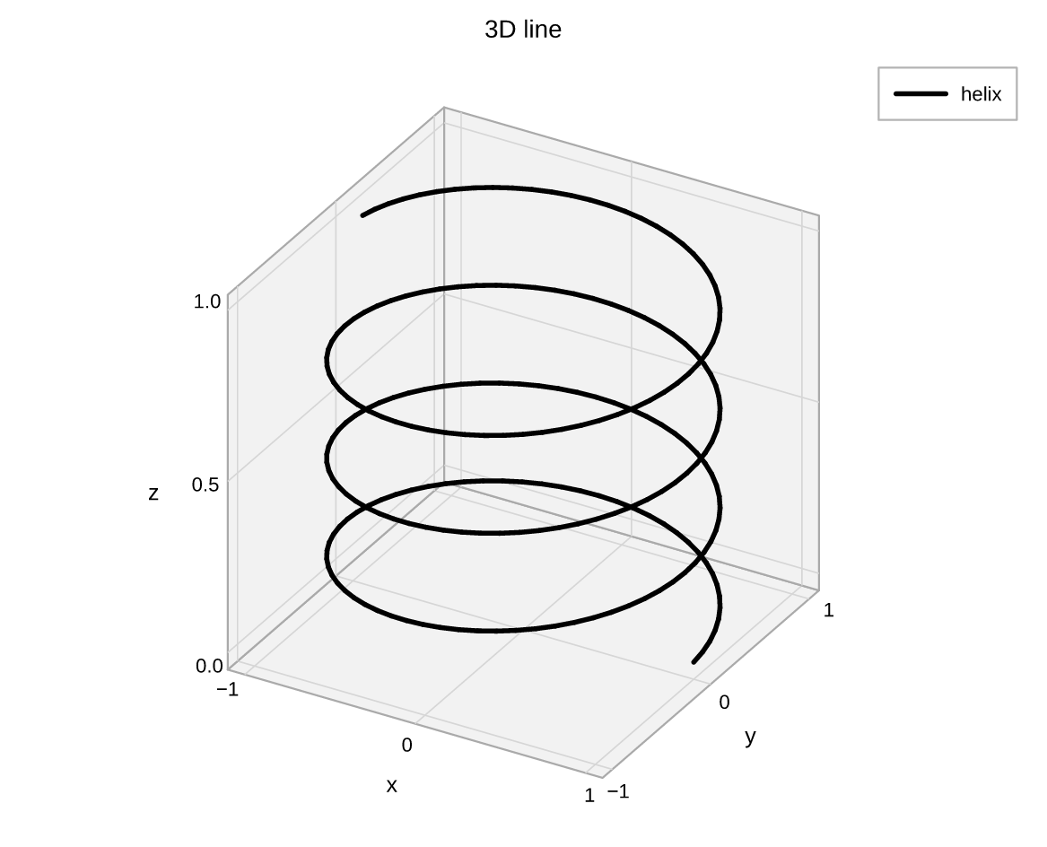
plot (alias plot3d) draws a 3D polyline:

"""A 3D parametric curve (helix)."""
import math

import pyplotrs as pp

t = [i * 0.1 for i in range(220)]
xs = [math.cos(v) for v in t]
ys = [math.sin(v) for v in t]
zs = [v / (22.0) for v in t]
fig, ax = pp.subplots(projection="3d", figsize=(420, 340))
ax.plot(xs, ys, zs, color="C0", linewidth=2.0, label="helix")
ax.set(title="3D line", xlabel="x", ylabel="y", zlabel="z")
ax.legend()
fig.save("line3d.png")

3D line

Scatter¶

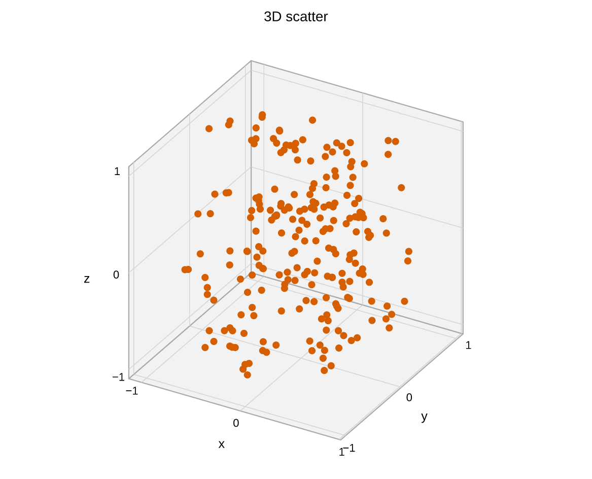
scatter (alias scatter3d) places depth-sorted markers:

"""3D scatter cloud."""
import math

import pyplotrs as pp


def rnd(seed):
    s = seed
    while True:
        s = (1103515245 * s + 12345) & 0x7FFFFFFF
        yield (s / 0x7FFFFFFF) * 2 - 1
g = rnd(7)
xs, ys, zs = [], [], []
for _ in range(220):
    t = next(g) * math.pi
    r = 0.6 + 0.4 * next(g)
    xs.append(r * math.cos(3 * t) + 0.1 * next(g))
    ys.append(r * math.sin(3 * t) + 0.1 * next(g))
    zs.append(t / math.pi)
fig, ax = pp.subplots(projection="3d", figsize=(420, 340))
ax.scatter(xs, ys, zs, color="C6", markersize=5.1)
ax.set(title="3D scatter", xlabel="x", ylabel="y", zlabel="z")
fig.save("scatter3d.png")

3D scatter

The rest of the vocabulary¶

Method	What it draws
`bar3d(x, y, z, dx, dy, dz)`	Boxes with base corner `(x, y, z)` and sizes `(dx, dy, dz)`, each a scalar or a per-bar array
`plot_wireframe(X, Y, Z)`	The grid as row and column lines
`contour3d(X, Y, Z, levels=…)`	Contour lines drawn at their z-heights, one color per level from `cmap`
`plot_trisurf(x, y, z)`	Surface over scattered points: Delaunay-triangulated in the `(x, y)` plane (or use your own `triangles=` index triples), each facet shaded by mean z
`quiver3d(x, y, z, u, v, w)`	Arrows `(u, v, w)` rooted at `(x, y, z)`, scaled by `length=`
`voxels(filled)`	A boolean occupancy grid `filled[i][j][k]` as unit cubes

Every 3D mark takes alpha and label. The colormapped kinds (surface, plot_trisurf, contour3d) have no single data color, so their legend key is a representative swatch — the colormap's midpoint, or the middle level.

Camera & labels¶

Set the view angle and axis labels through set:

ax.set(title="…", xlabel="x", ylabel="y", zlabel="z",
       elev=35, azim=-50, zlim=(0, 1))

elev is the angle above the x–y plane and azim the rotation about the vertical axis (degrees), matching matplotlib's mplot3d convention. Read them back with get_view(), and the limits with get_xlim() / get_ylim() / get_zlim().

Interactive HTML¶

Saving a 3D figure to .html produces a dependency-free Canvas2D viewer you can orbit (drag), zoom (scroll) and pan (shift-drag):

fig.save("surface.html")

The theme colors, tick labels and pre-sampled surface face colors travel with the page; nothing is fetched at view time.

Depth sorting

Surfaces, lines and points are depth-sorted within each group rather than merged into one global painter's order, so a line can occasionally draw over a surface bump it is technically behind. This is fine for typical scenes.

A figure is 2D or 3D, not both

projection="3d" applies to the whole subplots grid, and a figure's axes are homogeneous when saving to HTML (a 3D figure becomes the viewer, a 2D one becomes inline SVG). Mixing kinds in one figure via add_subplot works for the static formats.